Basic Consumption-Savings Model

This example demonstrates how to create and solve a basic consumption-savings model using scikit-agent. The model represents an agent who must decide how much to consume and save in each period to maximize lifetime utility.

This is a fundamental model in macroeconomics and serves as a building block for more complex economic models.

# Authors: scikit-agent team
# License: MIT

import numpy as np
import matplotlib.pyplot as plt

# For now, we'll create a simple placeholder example
# In the future, this would use actual scikit-agent classes

print(__doc__)

Model Setup

We start by setting up the parameters for our consumption-savings model. The agent lives for T periods and must decide in each period how much to consume versus save for the future.

# Model parameters
T = 50  # Number of periods
beta = 0.95  # Discount factor
sigma = 2.0  # Coefficient of relative risk aversion
r = 0.03  # Interest rate

# Initial wealth
W0 = 1.0

print("Model parameters:")
print(f"  Periods (T): {T}")
print(f"  Discount factor (β): {beta}")
print(f"  Risk aversion (σ): {sigma}")
print(f"  Interest rate (r): {r}")

Model parameters:
  Periods (T): 50
  Discount factor (β): 0.95
  Risk aversion (σ): 2.0
  Interest rate (r): 0.03

Solution Method

For this simple example, we’ll solve the model analytically. In practice, scikit-agent would provide numerical solution methods.

# Analytical solution for consumption in each period
def consumption_rule(t, W, T, beta, sigma, r):
    """
    Analytical consumption function for finite horizon problem.

    Parameters
    ----------
    t : int
        Current period
    W : float
        Current wealth
    T : int
        Total periods
    beta : float
        Discount factor
    sigma : float
        Risk aversion
    r : float
        Interest rate

    Returns
    -------
    float
        Optimal consumption in period t
    """
    # Simplified consumption rule (approximate)
    periods_left = T - t
    if periods_left > 0:
        # Consumption rate increases as we approach end of life
        consumption_rate = 1 / (1 + beta * periods_left)
        return consumption_rate * W
    else:
        return W  # Consume everything in last period

Simulation

Now we simulate the optimal consumption and wealth paths.

# Arrays to store results
consumption = np.zeros(T)
wealth = np.zeros(T + 1)
wealth[0] = W0

# Simulate the optimal path
for t in range(T):
    # Calculate optimal consumption
    consumption[t] = consumption_rule(t, wealth[t], T, beta, sigma, r)

    # Update wealth for next period
    if t < T - 1:
        wealth[t + 1] = (wealth[t] - consumption[t]) * (1 + r)

print("\nSimulation completed!")
print(f"Initial wealth: {wealth[0]:.3f}")
print(f"Final wealth: {wealth[T]:.3f}")
print(f"Average consumption: {np.mean(consumption):.3f}")

Simulation completed!
Initial wealth: 1.000
Final wealth: 0.000
Average consumption: 0.044

Visualization

Let’s plot the consumption and wealth paths over time.

fig, (ax1, ax2) = plt.subplots(2, 1, figsize=(10, 8))

# Plot consumption over time
ax1.plot(range(T), consumption, "b-", linewidth=2, label="Consumption")
ax1.set_xlabel("Period")
ax1.set_ylabel("Consumption")
ax1.set_title("Optimal Consumption Path")
ax1.grid(True, alpha=0.3)
ax1.legend()

# Plot wealth over time
ax2.plot(range(T + 1), wealth, "r-", linewidth=2, label="Wealth")
ax2.set_xlabel("Period")
ax2.set_ylabel("Wealth")
ax2.set_title("Wealth Evolution")
ax2.grid(True, alpha=0.3)
ax2.legend()

plt.tight_layout()
plt.show()

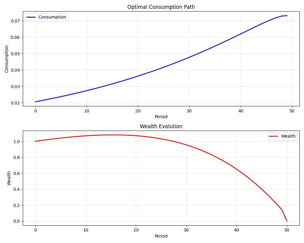
Analysis

The results show the typical pattern for a finite horizon consumption problem: consumption increases over time as the agent approaches the end of life, and wealth decreases correspondingly.

print("\nAnalysis:")
print(f"  Consumption in first period: {consumption[0]:.3f}")
print(f"  Consumption in last period: {consumption[-1]:.3f}")
print(f"  Total consumption: {np.sum(consumption):.3f}")
print(f"  Wealth depletion: {(W0 - wealth[T]) / W0 * 100:.1f}%")

Analysis:
  Consumption in first period: 0.021
  Consumption in last period: 0.073
  Total consumption: 2.181
  Wealth depletion: 100.0%