Consumption-Saving-Portfolio Model

The consumption-saving problem is one of the central models of modern macroeconomics and household finance. An agent with uncertain income must decide each period how much to consume and how much to save, trading off current utility against future resources.

This example uses the model blocks defined in skagent.models.consumer, which implements Carroll’s (2001) [1] formulation of the normalized buffer-stock problem and extends it with a portfolio choice between a safe bond and a risky asset.

Model Structure

The model is built from three composable blocks:

• consumption_block_normalized - one period of the normalized consumption-saving problem

• portfolio_block - risky portfolio allocation that endogenizes the gross return \(R\)

• tick_block - state transition that carries end-of-period assets into next period’s capital

The two complete recursive problems are:

• cons_problem - pure saving (fixed return)

• cons_portfolio_problem - saving plus portfolio choice

Normalized Consumption Block

State Variable: \(k_t\) - normalized capital (assets divided by permanent income) carried into the period

Shocks:

• \(\theta_t\) - transitory income shock, \(\mathbb{E}[\theta_t] = 1\)

Dynamics:

\[b_t = \frac{k_t R}{G}\]

\[m_t = b_t + \theta_t\]

\[c_t \in [0,\, m_t] \quad \text{(control)}\]

\[a_t = m_t - c_t\]

where \(G\) = PermGroFac is the permanent income growth factor and \(R\) is the gross return on savings.

Utility:

\[u(c_t) = \frac{c_t^{1-\rho}}{1-\rho}, \quad \rho = \text{CRRA}\]

Portfolio Block

The portfolio block augments the saving problem with an endogenous asset return. The agent chooses the risky share \(\varsigma_t \in [0,1]\):

\[R_t = R_f + (R^{\text{risky}}_t - R_f)\,\varsigma_t\]

where \(R^{\text{risky}}_t \sim \text{Lognormal}(R_f + \text{EqP},\, \text{RiskyStd})\).

Parameters

• \(\beta\) (DiscFac) = 0.96: Discount factor

• \(\rho\) (CRRA) = 2.0: Coefficient of relative risk aversion

• \(R\) = 1.03: Gross safe return (3 % per period)

• \(G\) (PermGroFac) = 1.01: Permanent income growth factor

• \(\sigma_\theta\) (TranShkStd) = 0.1: Transitory income shock std

• \(R_f\) (Rfree) = 1.03: Risk-free rate

• \(\text{EqP}\) = 0.02: Equity premium

• \(\sigma_R\) (RiskyStd) = 0.1: Risky return std

References

[1]

Carroll, C.D. (2001). “A Theory of the Consumption Function, With and Without Liquidity Constraints.” Journal of Economic Perspectives, 15(3), 23-45.

import matplotlib.pyplot as plt
import numpy as np
import skagent as ska
from skagent.distributions import Normal
import skagent.models.consumer as cons

Model Inspection

Load the predefined model elements and inspect them.

Step 1: Show Model Parameters

print("Model Calibration:")
for param, value in cons.calibration.items():
    print(f"  {param}: {value}")

Model Calibration:
  DiscFac: 0.96
  CRRA: 2.0
  R: 1.03
  Rfree: 1.03
  EqP: 0.02
  LivPrb: 0.98
  PermGroFac: 1.01
  TranShkStd: 0.1
  RiskyStd: 0.1
  kInitStd: 1
  pInitStd: 1

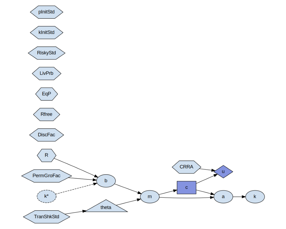
Step 2a: Inspect the Consumption Block Formulas

cons.cons_problem.display_formulas()

b = lambda k, R, PermGroFac: k * R / PermGroFac
m = lambda b, theta: b + theta
c = Control(m)
a = lambda m, c: m - c
u = lambda c, CRRA: torch.log(c
k = lambda a: a

Step 2b: Visualize the Consumption Block

img, _ = cons.cons_problem.display(cons.calibration)

plt.figure(figsize=(10, 8))
plt.imshow(img)
plt.axis("off")
plt.tight_layout()

<IPython.core.display.SVG object>

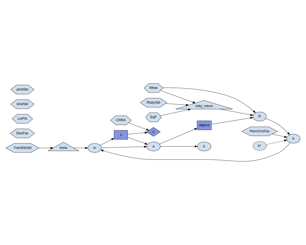
Step 3a: Inspect and visualize the Portfolio Block

cons.cons_portfolio_problem.display_formulas()

b = lambda k, R, PermGroFac: k * R / PermGroFac
m = lambda b, theta: b + theta
c = Control(m)
a = lambda m, c: m - c
u = lambda c, CRRA: torch.log(c
stigma = Control(a)
R = lambda stigma, Rfree, risky_return: Rfree
k = lambda a: a

Step 3b: Inspect and visualize the Portfolio Block

img, _ = cons.cons_portfolio_problem.display(cons.calibration)

plt.figure(figsize=(10, 8))
plt.imshow(img)
plt.axis("off")
plt.tight_layout()

<IPython.core.display.SVG object>

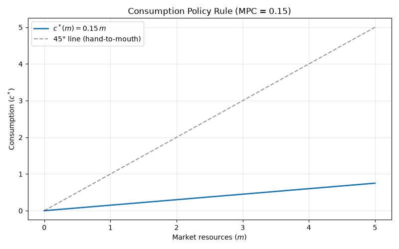
Step 4: Define a Simple Consumption Rule

The optimal policy for this model requires numerical solution methods. Here we use a simple constant marginal propensity to consume (MPC) rule as a tractable approximation:

\[c^*(m) = \kappa \cdot m\]

where \(\kappa \in (0, 1)\) is a fixed MPC. A low MPC creates buffer-stock saving behaviour: agents accumulate assets and consume out of wealth gradually.

MPC = 0.15  # Marginal propensity to consume


def consumption_rule(m):
    """Consume a fixed fraction of market resources each period."""
    return MPC * m


decision_rule = {"c": consumption_rule}

# Plot the consumption rule
m_range = np.linspace(0, 5, 200)
plt.figure(figsize=(8, 5))
plt.plot(m_range, consumption_rule(m_range), linewidth=2, label=rf"$c^*(m) = {MPC}\,m$")
plt.plot(m_range, m_range, "k--", alpha=0.4, label="45° line (hand-to-mouth)")
plt.xlabel("Market resources ($m$)")
plt.ylabel("Consumption ($c^*$)")
plt.title(f"Consumption Policy Rule (MPC = {MPC})")
plt.legend()
plt.grid(True, alpha=0.3)
plt.tight_layout()

Step 5: Run Monte Carlo Simulation (Pure Saving Problem)

Simulate the pure saving problem (cons_problem) which combines the normalized consumption block with the tick block. Agents start with normalized capital \(k \approx 1\).

initial_conditions = {
    "k": Normal(mu=1.0, sigma=0.1),
}

simulator = ska.MonteCarloSimulator(
    calibration=cons.calibration.copy(),
    block=cons.cons_problem,
    dr=decision_rule,
    initial=initial_conditions,
    agent_count=1000,
    T_sim=100,
    seed=42,
)

print("\nRunning simulation...")
simulator.initialize_sim()
simulator.simulate()
print("Simulation completed successfully")

Running simulation...
Simulation completed successfully

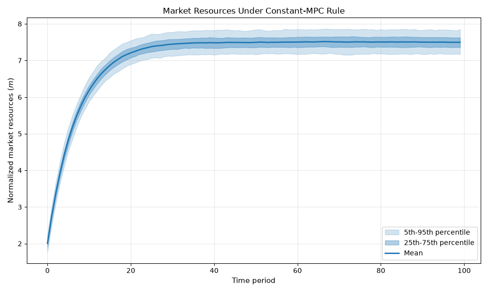
Step 6: Plot Simulation Results

The plot shows the cross-sectional distribution of normalized market resources \(m_t\) over time. Under the constant-MPC rule, agents accumulate a buffer stock of savings that stabilizes around a long-run mean determined by \(\kappa\), \(R\), and \(G\).

plt.figure(figsize=(10, 6))

m_hist = simulator.history["m"]

plt.fill_between(
    range(simulator.T_sim),
    np.percentile(m_hist, 5, axis=1),
    np.percentile(m_hist, 95, axis=1),
    alpha=0.2,
    color="C0",
    label="5th-95th percentile",
)
plt.fill_between(
    range(simulator.T_sim),
    np.percentile(m_hist, 25, axis=1),
    np.percentile(m_hist, 75, axis=1),
    alpha=0.35,
    color="C0",
    label="25th-75th percentile",
)
plt.plot(m_hist.mean(axis=1), linewidth=2, color="C0", label="Mean")

plt.xlabel("Time period", fontsize=11)
plt.ylabel("Normalized market resources ($m$)", fontsize=11)
plt.title("Market Resources Under Constant-MPC Rule", fontsize=12)
plt.legend(fontsize=10)
plt.grid(True, alpha=0.3)
plt.tight_layout()
plt.show()

Step 7: Run Portfolio Simulation

Now extend to the portfolio problem (cons_portfolio_problem), where agents also choose their risky asset share \(\varsigma_t\). We pair the MPC consumption rule with a fixed risky share of 0.5.

RISKY_SHARE = 0.5  # Fixed portfolio share in risky asset

portfolio_decision_rule = {
    "c": consumption_rule,
    "stigma": lambda a: RISKY_SHARE,
}

portfolio_sim = ska.MonteCarloSimulator(
    calibration=cons.calibration.copy(),
    block=cons.cons_portfolio_problem,
    dr=portfolio_decision_rule,
    initial={"k": Normal(mu=1.0, sigma=0.1), "R": cons.calibration["Rfree"]},
    agent_count=1000,
    T_sim=100,
    seed=42,
)

print("\nRunning portfolio simulation...")
portfolio_sim.initialize_sim()
portfolio_sim.simulate()
print("Portfolio simulation completed successfully")

Running portfolio simulation...
Portfolio simulation completed successfully

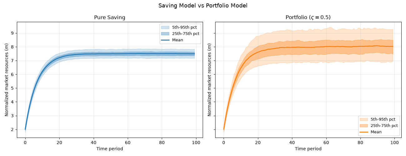
Step 8: Compare Saving vs Portfolio Paths

The risky asset earns a higher expected return, so the portfolio model predicts higher mean wealth accumulation - but also greater dispersion due to stock-return risk.

fig, axes = plt.subplots(1, 2, figsize=(13, 5), sharey=True)
fig.suptitle("Saving Model vs Portfolio Model", fontsize=13)

for ax, sim, label, color in [
    (axes[0], simulator, "Pure Saving", "C0"),
    (axes[1], portfolio_sim, rf"Portfolio ($\varsigma={RISKY_SHARE}$)", "C1"),
]:
    m_h = sim.history["m"]
    ax.fill_between(
        range(sim.T_sim),
        np.percentile(m_h, 5, axis=1),
        np.percentile(m_h, 95, axis=1),
        alpha=0.2,
        color=color,
        label="5th-95th pct",
    )
    ax.fill_between(
        range(sim.T_sim),
        np.percentile(m_h, 25, axis=1),
        np.percentile(m_h, 75, axis=1),
        alpha=0.35,
        color=color,
        label="25th-75th pct",
    )
    ax.plot(m_h.mean(axis=1), linewidth=2, color=color, label="Mean")
    ax.set_title(label)
    ax.set_xlabel("Time period")
    ax.set_ylabel("Normalized market resources ($m$)")
    ax.legend(fontsize=9)
    ax.grid(True, alpha=0.3)

plt.tight_layout()
plt.show()