Resource Extraction Model

The resource extraction problem models the optimal management of a renewable resource (fishery, forest, wildlife, etc.). The decision-maker must balance immediate profits from extraction against preserving the resource stock for future use.

This example implements the classic model from Reed (1979) [1], which shows that under multiplicative environmental shocks and stock-dependent harvesting costs, the optimal policy has a simple “constant escapement” form. The optimal escapement level can be computed analytically, making this an excellent benchmark for testing reinforcement learning algorithms.

Model Structure

• State Variable: \(x_t\) — Resource stock level at time \(t\)

• Control Variable: \(u_t\) — Harvest/extraction rate (constrained: \(0 \leq u_t \leq x_t\))

Dynamics

The resource stock evolves according to:

\[x_{t+1} = r(x_t - u_t) \epsilon_t\]

where:

• \(r > 1\) is the deterministic growth rate

• \((x_t - u_t)\) is the escapement (stock remaining after harvest)

• \(\epsilon_t\) is a multiplicative environmental shock with \(\mathbb{E}[\epsilon_t] = 1\)

• \(\epsilon_t\) follows a log-normal distribution: \(\ln(\epsilon_t) \sim \mathcal{N}(-\sigma^2/2, \sigma^2)\)

Profit Function

Single-period profit is:

\[\pi(u_t, x_t) = \left(p - \frac{c_0}{x_t}\right) u_t\]

where:

• \(p\) is the (constant) price per unit harvested

• \(c_0/x_t\) is the stock-dependent unit cost of harvesting

The cost specification captures the realistic feature that harvesting becomes more expensive when the stock is depleted (e.g., fish are harder to catch when populations are low).

Objective and Bellman Equation

The manager seeks to maximize expected discounted profit:

\[V(x_t) = \max_{u_t} \mathbb{E}\left[\pi(u_t, x_t) + \delta V(x_{t+1})\right]\]

where \(\delta \in (0,1)\) is the discount factor, which reflects time preference (impatience) and risk. The Bellman equation expresses the value of being in state \(x_t\) as the maximum of current profit plus the discounted expected continuation value.

Parameters

• \(r\) = 1.1: Growth rate (10% per period)

• \(p\) = 5.0: Price per unit extracted

• \(c_0\) = 2.0: Cost parameter for stock-dependent costs

• \(\delta\) (DiscFac) = 0.95: Discount factor for future rewards

• \(\sigma\) = 0.1: Standard deviation of log-normal growth shock

Optimal Policy: Constant Escapement

Reed (1979) [1] proved that the optimal policy maintains a constant target stock level \(S^*\) and harvests any surplus:

\[u_t^* = \max(0, x_t - S^*)\]

The optimal escapement level is:

\[S^* = \frac{c_0 (1 - \delta)}{p (1 - \delta r)}\]

This requires the “impatience condition” \(\delta r < 1\), which ensures the agent prefers extraction over indefinite accumulation.

References

[1] (1,2)

Reed, W.J. (1979). “Optimal escapement levels in stochastic and deterministic harvesting models.” Journal of Environmental Economics and Management, 6(4), 350-363.

import matplotlib.pyplot as plt
import numpy as np
import skagent as ska
from skagent.distributions import Normal
import skagent.models.resource_extraction as rex

Model Inspection

First, let’s load the predefined model elements and inspect them.

Step 1: Show Model Parameters

print("Model Calibration:")
for param, value in rex.calibration.items():
    print(f"  {param}: {value}")

Model Calibration:
  r: 1.02
  p: 5.0
  c_0: 10.0
  DiscFac: 0.95
  sigma: 0.1

Step 2: Inspect the Resource Extraction Model

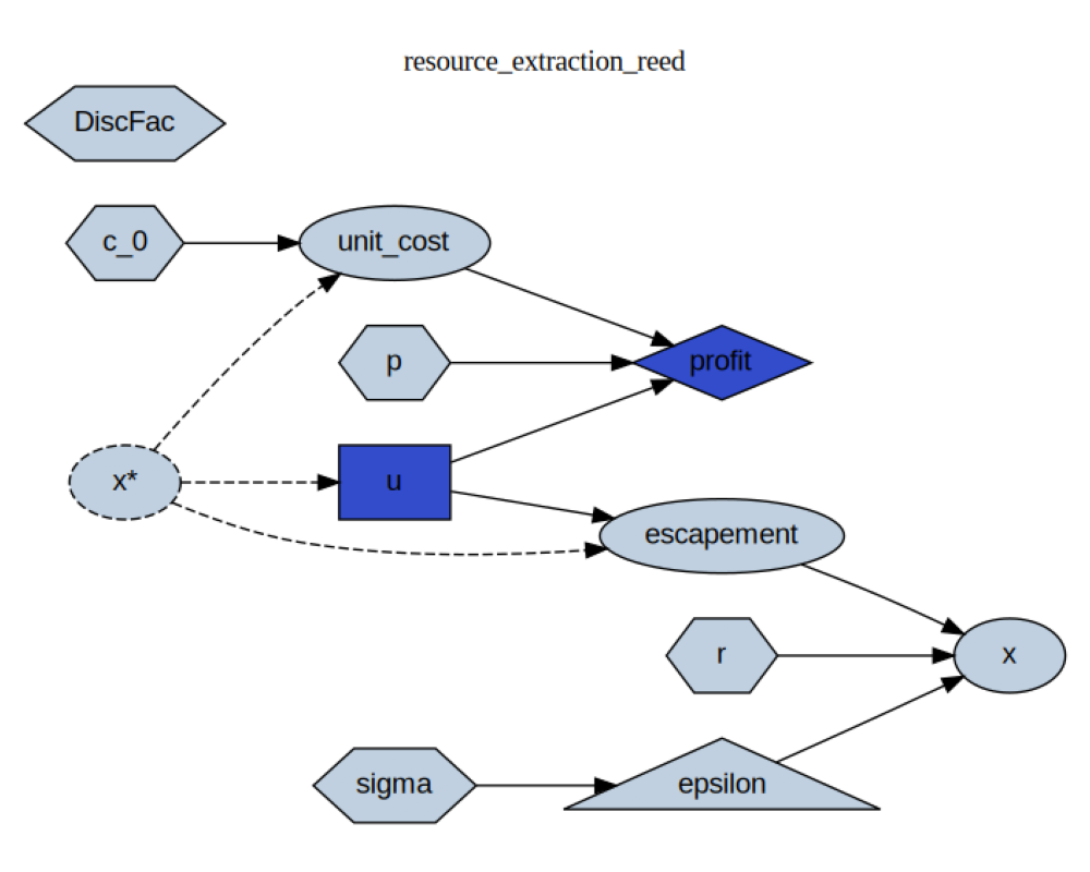
rex.resource_extraction_block.display_formulas()

u = Control(x)
unit_cost = lambda x, c_0: c_0 / x
profit = lambda u, p, unit_cost: (p - unit_cost) * u
escapement = lambda x, u: x - u
x = lambda escapement, r, epsilon: r * escapement * epsilon

Step 3: Visualize the Resource Extraction Model

img, _ = rex.resource_extraction_block.display(rex.calibration)

plt.figure(figsize=(10, 8))
plt.imshow(img)
plt.axis("off")
plt.tight_layout()

<IPython.core.display.SVG object>

Step 4: Compute Optimal Escapement Policy

Reed (1979) proved that the optimal policy has a constant escapement form:

\[u^*(x) = \max(0, x - S^*)\]

where \(S^*\) is the optimal escapement level (target stock to maintain).

The optimal escapement can be computed analytically:

\[S^* = \frac{c_0 (1 - \delta)}{p (1 - \delta r)}\]

This analytical solution makes the model ideal for validating reinforcement learning algorithms—we can compare learned policies against the known optimum.

dr_u, _ = rex.make_optimal_decision_rule(rex.calibration)

# Compute S* for display
r = rex.calibration["r"]
p = rex.calibration["p"]
c_0 = rex.calibration["c_0"]
delta = rex.calibration["DiscFac"]
S_star = c_0 * (1 - delta) / (p * (1 - delta * r))

print(f"\nOptimal escapement level: S* = {S_star:.4f}")
print(f"Optimal policy: u*(x) = max(0, x - {S_star:.4f})")

# Visualize the policy
x_range = np.linspace(0, 5, 100)
u_optimal = dr_u(x_range)

plt.figure(figsize=(8, 5))
plt.plot(x_range, u_optimal, label=r"$u^*(x) = \max(0, x - S^*)$", linewidth=2)
plt.axhline(y=0, color="k", linestyle="--", alpha=0.3)
plt.axvline(
    x=S_star, color="r", linestyle="--", alpha=0.5, label=f"$S^* = {S_star:.2f}$"
)
plt.xlabel("Stock level (x)")
plt.ylabel("Optimal harvest (u*)")
plt.title("Reed's Constant Escapement Policy")
plt.legend()
plt.grid(True, alpha=0.3)
plt.tight_layout()

# Wrap rules in the format expected by simulator
decision_rule = {"u": dr_u}

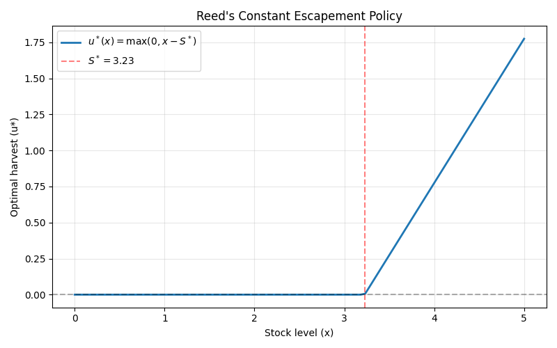
Optimal escapement level: S* = 3.2258
Optimal policy: u*(x) = max(0, x - 3.2258)

Step 5: Run Monte Carlo Simulation

# Initial conditions - start with stock level around 2*S*
initial_conditions = {
    "x": Normal(mu=2 * S_star, sigma=0.1),
}

# Create and run simulator
simulator = ska.MonteCarloSimulator(
    calibration=rex.calibration,
    block=rex.resource_extraction_block,
    dr=decision_rule,
    initial=initial_conditions,
    agent_count=1000,  # Simulate 1000 agents
    T_sim=100,  # For 100 periods
    seed=42,  # For reproducibility
)

# Run the simulation
print("\nRunning simulation...")
simulator.initialize_sim()  # Initialize simulation variables
simulator.simulate()

print("✓ Simulation completed successfully")

Running simulation...
✓ Simulation completed successfully

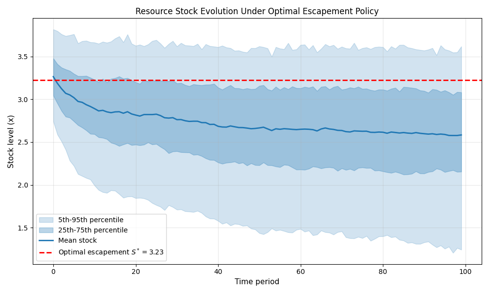
Step 6: Plot Simulation Results

The plot shows the distribution of stock levels over time under the optimal constant escapement policy. The stock fluctuates around \(S^*\) due to environmental shocks. When stock exceeds \(S^*\), the surplus is harvested; when shocks drive stock below \(S^*\), no harvest occurs and the stock recovers through natural growth.

plt.figure(figsize=(10, 6))

# Plot percentiles to show distribution
plt.fill_between(
    range(simulator.T_sim),
    np.percentile(simulator.history["x"], 5, axis=1),
    np.percentile(simulator.history["x"], 95, axis=1),
    alpha=0.2,
    label="5th-95th percentile",
    color="C0",
)
plt.fill_between(
    range(simulator.T_sim),
    np.percentile(simulator.history["x"], 25, axis=1),
    np.percentile(simulator.history["x"], 75, axis=1),
    alpha=0.3,
    label="25th-75th percentile",
    color="C0",
)
plt.plot(
    simulator.history["x"].mean(axis=1), label="Mean stock", linewidth=2, color="C0"
)

# Add reference line for optimal escapement
plt.axhline(
    y=S_star,
    color="r",
    linestyle="--",
    linewidth=2,
    label=f"Optimal escapement $S^* = {S_star:.2f}$",
)

plt.xlabel("Time period", fontsize=11)
plt.ylabel("Stock level (x)", fontsize=11)
plt.title("Resource Stock Evolution Under Optimal Escapement Policy", fontsize=12)
plt.legend(fontsize=10)
plt.grid(True, alpha=0.3)
plt.tight_layout()
plt.show()