Training a Policy Network Against a Known Solution

This example demonstrates scikit-agent’s neural-network training pipeline by solving a model whose optimal policy is known in closed form, then comparing the trained policy against that analytical solution. Validating a solver against a known answer is the cleanest way to build trust in it before applying it to models that have no closed form.

The model: normalized permanent-income consumption (U-2)

The U-2 benchmark is a normalized version of the permanent-income hypothesis (PIH) consumption-savings problem. It is one of the analytic benchmarks in skagent.models.benchmarks; that module’s registry holds the full block definition, the calibration, and the closed-form policy (get_analytical_policy()) used as the target below. Working in ratios to permanent income, the state is normalized assets \(a\), the within-period resource is cash-on-hand \(m = R a / \psi + 1\), and the control is normalized consumption \(c\). The agent solves

\[V(m) = \max_{c} \; u(c) + \beta \, \mathbb{E}\!\left[ V(m') \right],\]

with constant-relative-risk-aversion utility \(u\) and discount factor \(\beta\). For this calibration the optimal policy is affine in cash-on-hand,

\[c^*(m) = \kappa \, (m + h),\]

where both the marginal propensity to consume \(\kappa = 1 - \beta\) and the normalized human wealth \(h = 1/r\) have closed forms. At this calibration \(h = 1/0.03 \approx 33.3\), so the intercept \(\kappa h\) dominates and the consumption function is nearly flat over the training range. This gives us an exact target to check the trained policy against.

Why a value head: the level-identification problem

A policy trained only on the Euler equation \(u'(c_t) = \beta R \, \mathbb{E}[u'(c_{t+1})]\) pins down the slope of the consumption function but not its level: scaling the whole policy leaves the Euler residual nearly unchanged. A BlockPolicyValueNet resolves this indeterminacy: it shares one hidden backbone between a policy head and a value head, training them together under a single optimizer with BellmanEquationLoss. The value head anchors the level through the Bellman equation \(V(m) = u(c) + \beta \mathbb{E}[V(m')]\), which pins down what the Euler equation alone leaves free.

Why we re-sample the states

The single most important ingredient for accuracy is that the training states are re-sampled on every gradient step, not fixed once. Maliar, Maliar, and Winant (2021) keep the data “constantly re-sampled during training,” and it matters: on a fixed handful of points the network drives those points’ residuals to zero while the consumption level drifts between them, and the error stalls at several percent (and worsens with more epochs). Drawing a fresh batch each step instead enforces the residual across the whole domain, which pins the level and lets the error fall below one percent. The per-step optimizer is train_block_nn(); the loop in Step 4 supplies the fresh states and threads Adam’s momentum through. The loss combines the MMW’21 all-in-one expectation operator (two independent shock copies per state) with the Bellman first-order-condition term.

A complementary ingredient of the full MMW’21 algorithm, simulating the model forward so the sampled states concentrate on the ergodic set, is provided by maliar_training_loop(); for a worked demonstration on a model with no closed-form solution, see the companion gallery example plot_maliar_training_loop.py.

import matplotlib.pyplot as plt
import numpy as np
import torch

import skagent.bellman as bellman
import skagent.grid as grid
import skagent.loss as loss
from skagent.ann import BlockPolicyValueNet, device, train_block_nn
from skagent.models.benchmarks import (
    get_analytical_policy,
    get_benchmark_calibration,
    get_benchmark_model,
)

SEED = 10077693

Step 1: Load the U-2 benchmark and build a BellmanPeriod

get_benchmark_model returns the model block; get_analytical_policy returns the closed-form solution we will validate against.

u2_block = get_benchmark_model("U-2")
u2_calibration = get_benchmark_calibration("U-2")
analytical_policy = get_analytical_policy("U-2")

rng = np.random.default_rng(SEED)
u2_block.construct_shocks(u2_calibration, rng=rng)

bp = bellman.BellmanPeriod(u2_block, "DiscFac", u2_calibration)

Step 2: Build the shared-backbone policy/value network

A single BlockPolicyValueNet carries both a (bounded) policy head and an unconstrained value head on top of one shared hidden stack. One optimizer updates all of its weights together.

torch.manual_seed(SEED)
pvnet = BlockPolicyValueNet(bp, width=32)

Step 3: Define the Bellman-equation loss

BellmanEquationLoss evaluates the residual of \(V(m) = u(c) + \beta \mathbb{E}[V(m')]\) using the network’s own value head. foc_weight=1.0 adds the first-order-condition term (Maliar et al. 2021, eq. 14), which speeds convergence.

bellman_loss_fn = loss.BellmanEquationLoss(
    bp,
    pvnet.get_value_function(),
    parameters=u2_calibration,
    foc_weight=1.0,
)

Step 4: Train on re-sampled states, snapshotting at increasing depths

Accuracy hinges on re-sampling the training states on every gradient step rather than fixing a grid (Maliar et al. 2021, who keep the data “constantly re-sampled during training”). A fresh draw each step enforces the residual across the whole domain; a fixed handful of points lets the network drive their residuals to zero while the consumption level drifts between them. Each step draws n_batch normalized-asset points with two independent permanent-income shock copies (the all-in-one operator), and threads the optimizer back in so Adam keeps its momentum across steps.

We evaluate the policy on a fixed grid at several training depths, so the plot can show the consumption function converging toward the analytical solution as training proceeds rather than only its final fit. The depths are checkpoints of one continuous run (the optimizer is threaded through), so snapshotting only observes training, it does not perturb it.

# Evaluation grid, held fixed across depths. The income shock is held at its
# mean so the slice is deterministic; cash-on-hand is then m = R a + 1.
n_test = 50
test_a = torch.linspace(0.5, 5.0, n_test, device=device)
test_states = {"a": test_a}
test_shocks = {"psi": torch.ones(n_test, device=device)}
test_m = (u2_calibration["R"] * test_a / test_shocks["psi"] + 1.0).cpu().numpy()


def consumption_on_test_grid(net):
    decision_fn = net.get_decision_function()
    c = decision_fn(test_states, test_shocks, u2_calibration)["c"]
    return c.detach().cpu().numpy()


n_batch = 256
checkpoints = [100, 500, 1500, 5000]  # cumulative SGD steps to snapshot at
snapshots = {}
optimizer = None
final_loss = float("nan")
step = 0
for target in checkpoints:
    while step < target:
        train_grid = grid.Grid.from_dict(
            {
                "a": torch.empty(n_batch, device=device).uniform_(0.5, 5.0),
                "psi_0": torch.ones(n_batch, device=device),
                "psi_1": torch.ones(n_batch, device=device),
            }
        )
        pvnet, final_loss, optimizer = train_block_nn(
            pvnet,
            train_grid,
            bellman_loss_fn,
            epochs=1,
            lr=1e-3,
            optimizer=optimizer,
            verbose=False,
        )
        step += 1
    snapshots[target] = consumption_on_test_grid(pvnet)
trained_net = pvnet
print(f"Final training loss: {final_loss:.3e}")

Final training loss: 3.487e-06

Step 5: Compare the deepest-trained policy to the analytical solution

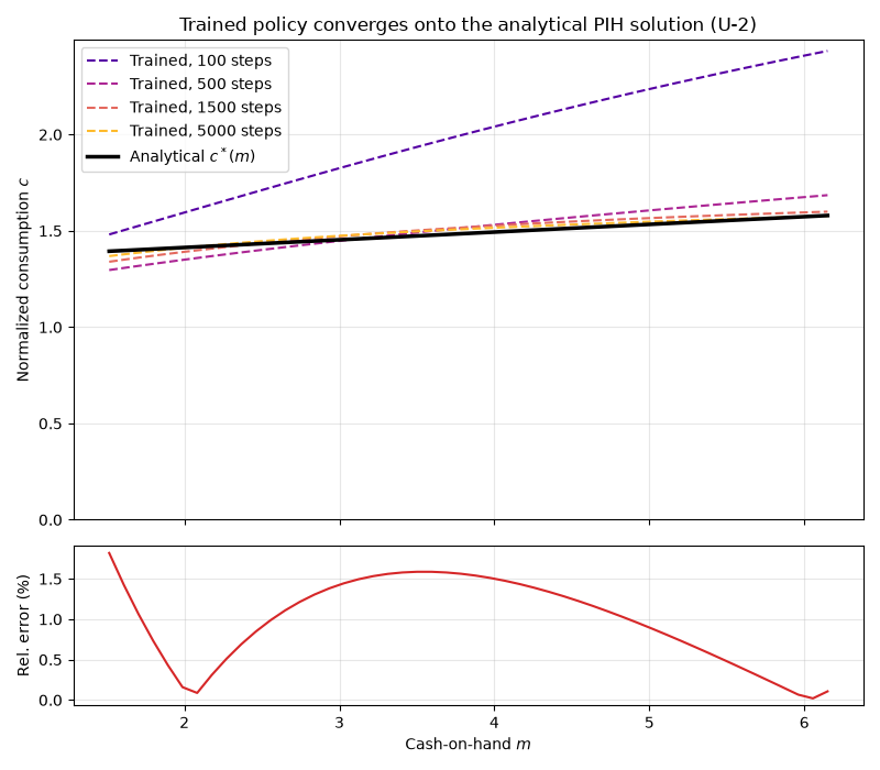
At the deepest snapshot we report the pointwise relative error against the closed-form policy. With re-sampled training and the value head anchoring the level, the mean relative error falls to about one percent (here 0.98%), an order of magnitude tighter than the several-percent floor of Euler-only training on this unconstrained model.

analytical_np = (
    analytical_policy(test_states, test_shocks, u2_calibration)["c"]
    .detach()
    .cpu()
    .numpy()
)
trained_np = snapshots[checkpoints[-1]]

rel_error_np = np.abs(trained_np - analytical_np) / (analytical_np + 1e-8)
print(f"Mean relative error:  {rel_error_np.mean():.2%}")
print(f"Max  relative error:  {rel_error_np.max():.2%}")

Mean relative error:  0.98%
Max  relative error:  1.82%

Step 6: Plot the policy converging onto the analytical solution

Consumption is a function of cash-on-hand m, so we plot against m (not assets a), and start the consumption axis at 0 so the level is shown honestly. Each dashed curve is the trained policy after a given number of SGD steps: as training deepens the curves march onto the closed-form linear PIH rule, making it visible that the error keeps shrinking with training rather than stalling. The lower panel shows the pointwise relative error at the deepest snapshot.

fig, (ax_policy, ax_err) = plt.subplots(
    2, 1, figsize=(8, 7), sharex=True, height_ratios=[3, 1]
)

depth_colors = plt.cm.plasma(np.linspace(0.15, 0.85, len(checkpoints)))
for color, steps in zip(depth_colors, checkpoints):
    ax_policy.plot(
        test_m,
        snapshots[steps],
        "--",
        color=color,
        linewidth=1.5,
        label=f"Trained, {steps} steps",
    )
ax_policy.plot(test_m, analytical_np, "k-", linewidth=2.5, label="Analytical $c^*(m)$")
ax_policy.set_ylabel("Normalized consumption $c$")
ax_policy.set_ylim(bottom=0.0)
ax_policy.set_title("Trained policy converges onto the analytical PIH solution (U-2)")
ax_policy.legend()
ax_policy.grid(True, alpha=0.3)

ax_err.plot(test_m, rel_error_np * 100.0, "C3-", linewidth=1.5)
ax_err.set_xlabel("Cash-on-hand $m$")
ax_err.set_ylabel("Rel. error (%)")
ax_err.grid(True, alpha=0.3)

fig.tight_layout()
plt.show()